Loopy Particle Math  

The Large Hadron Collider, or LHC, is the biggest machine humans have ever built. Pooling the resources of more than 100 countries, it accelerates protons to within a millionth of a percent of the speed of light. When they collide, the protons break into their component parts (quarks and the gluon particles that glue them together) and create particles that were not there before. This is how, in 2012, the LHC achieved the first detection of a Higgs boson, the final missing particle predicted by the Standard Model of particle physics. Now physicists hope the LHC will find something genuinely new: particles not already in their current theory—particles that explain the mystery of dark matter, for instance, or offer solutions to other lingering questions. For such a discovery, scientists must pore through the 30 petabytes a year of data the machine produces to identify tiny deviations where the results do not quite match the Standard Model.

Of course, all of that effort will be useless if we do not know what the Standard Model predicts.

That is where I come in. The questions we want to ask about the LHC come in the form of probabilities. “What is the chance that two protons bounce off each other?” “How often will we produce a Higgs boson?” Scientists compute these probabilities with “scattering amplitudes,” formulas that tell us how likely it is that particles “scatter” (essentially, bounce) off each other in a particular way. I am part of a group of physicists and mathematicians who work to speed up these calculations and find better tricks than the old, cumbersome methods handed down by our scientific forebears. We call ourselves “amplitudeologists.”

On supporting science journalism

If you're enjoying this article, consider supporting our award-winning journalism by subscribing. By purchasing a subscription you are helping to ensure the future of impactful stories about the discoveries and ideas shaping our world today.

Amplitudeologists trace our field back to the research of two physicists, Stephen Parke and Tomasz Taylor. In 1986 they found a single formula that described collisions between any number of gluons, simplifying what would ordinarily be pages of careful case-by-case calculations. The field actually kicked off in the 1990s and early 2000s, when a slew of new methods promised to streamline a wide variety of particle physics computations. Nowadays amplitudeology is booming: the Amplitudes 2018 conference had 160 participants, and 100 attended the summer school the week before, aimed at training young researchers in the tricks of the field. We have gotten some public attention, too: physicists Nima Arkani-Hamed and Jaroslav Trnka’s Amplituhedron (a way to describe certain amplitudes in the language of geometry) made the news in 2013, and on television The Big Bang Theory’s Sheldon Cooper has been known to dabble in amplitudeology.

Lately we have taken a big step forward, moving beyond the basic tools we have already developed into more complex techniques. We are entering a realm of calculations sensitive enough to match the increasing precision of the LHC. With these new tools we stand ready to detect even tiny differences between Standard Model predictions and the reality inside the LHC, potentially allowing us to finally reveal the undiscovered particles physicists dream of.

Loops and lines

To organize our calculations, scientists have long used pictures called Feynman diagrams. Invented by physicist Richard Feynman in 1948, these figures depict paths along which particles travel. Suppose we want to know the chance that two gluons merge and form a Higgs boson. We start by drawing lines representing the particles we know about: two gluons going in and one Higgs boson coming out. We then have to connect those lines by drawing more particle lines in the middle of the diagram, according to the rules of the Standard Model. These additional particles may be “virtual”: that is, they are not literally particles in the way the gluons and Higgs are in our picture. Instead they are shorthand, a way to keep track of how different quantum fields can interact.

Feynman diagrams are not just pretty pictures—they are instructions, telling us to use information about the particles we draw to calculate a probability. If we know the speed and energy of the gluons and Higgs boson in our diagram, we can try to work out the properties of the virtual particles in between. Sometimes, though, the answer is uncertain. Trace your finger along the particle paths, and you might find a closed loop: a path that ends up back where you started. A particle traveling in a loop like that is not “input” or “output”: its properties never get measured. We do not know how fast it is going or how much energy it has. Though counterintuitive, it is a consequence of the fundamental uncertainty of quantum mechanics, which prevents us from measuring two traits of a particle, such as speed and position, at the same time. Quantum mechanics tells us how to deal with this uncertainty—we have to add up every possibility, summing the probabilities for any speed and energy the virtual particles could have, using a technique you might remember from high school calculus: an integral.

In principle, to calculate a scattering amplitude we have to draw every diagram that could possibly connect our particles, every way the starting ingredients could have turned into the finished products (here the pair of gluons and the Higgs boson). That is a lot of diagrams, an infinite number, in fact: we could keep drawing loops inside loops as far as we like, requiring us to calculate more and more complicated integrals each time.

In practice, we are saved by the low strength of most quantum forces. When a group of lines in a diagram connect, it depicts an “interaction” among different types of particles. Each time this happens we have to multiply by a constant, related to the strength of the force that makes the particles interact. If we want to draw a diagram with more closed loops, we have to connect up more lines and multiply by more of these constants. For electricity and magnetism, the relevant constants are small: for each loop you add, you divide by roughly 137. This means that the diagrams with more and more loops make up a smaller and smaller piece of your final answer, and eventually that piece is so small that the experiments cannot detect it. The most careful experiments on electricity and magnetism are accurate up to an astounding 10 decimal places, some of the most precise measurements in all of science. Getting that far requires “only” four loops, four factors of 1/137 before the number you are calculating is too small to measure. In many cases, these numbers have actually been calculated, and all 10 decimal places agree with experiments.

The strong nuclear force is a tougher beast. It is the force that glues together protons and neutrons and the quarks inside them. It is quite a bit stronger than electricity and magnetism: for calculations at the LHC, each loop means dividing not by 137 but by 10. Getting up to 10 digits of precision would mean drawing 10 loops.

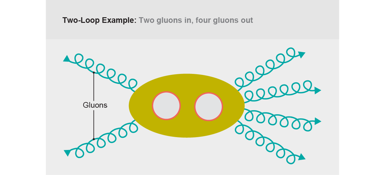
The LHC is not as precise as those electricity and magnetism experiments. At the moment, measurements from the machine are just starting to match the precision of two-loop calculations. Still, those results are already quite messy. For example, a two-loop calculation in 2010 by physicists Vittorio Del Duca, Claude Duhr and Vladimir Smirnov computed the chance that two gluons collide and four gluons come out. They made their calculation using a simplified theory, with some special shortcuts, and the resulting formula still clocked in at 17 pages of complicated integrals. That length was not too surprising; everyone knew that two-loop calculations were hard.

Until a few months later, when another group managed to write the same result on two lines. That group was a collaboration among three physicists—Marcus Spradlin, Cristian Vergu and Anastasia Volovich—and a mathematician, Alexander B. Goncharov. The trick they used was extraordinarily powerful, and it exposed amplitudeologists to an area of mathematics that most of us had not seen before, one that has driven my career to this day.

Periods and logs

Show a mathematician like Goncharov one of the integrals we get out of Feynman diagrams, and the first thing you will hear is, “That’s a period.”

Periods are a type of number. You might be familiar with the natural numbers (1, 2, 3, 4 ...) and the rational numbers (fractions). The square root of 2 is not rational—you cannot get it by dividing two natural numbers. What it is, though, is algebraic: you can write an algebraic equation, say x² = 2, where the square root of 2 is the solution. Periods are the next step up: although you cannot always get them from an algebraic equation, you can always get them from an integral.

Why call them periods? In the simplest cases, that is literally what they are: the distance before something repeats. Thinking back to high school, you might remember grappling with sines and cosines. You might even remember that you can put them together with imaginary numbers (the square roots of negative numbers—in other words, numbers that would not normally exist) using Euler’s formula: e^ix = cos (x) + i sin (x) (here e is a constant, and i is the square root of −1). All three of these—sin (x), cos (x), and e^ix—have period 2π: if you let x go from 0 to 2π, the function repeats, and you get the same numbers again.

2π is a period because it is the distance before e^ix repeats, but you can also think of it as an integral. Draw a graph of e^ix in the complex plane: imaginary numbers on one axis; real numbers on the other. It forms a circle. If you want to measure the length of that circle, you can do it with an integral, adding up each little segment all the way around. In doing so, you will find exactly 2π.

What happens if you go partway around the circle, to some point z? In that case, you must solve the equation z = e^ix. Thinking back again to high school, you might remember what you need to solve that equation: the natural logarithm, ln (z). Logarithms might not look like “periods” in the way 2π does, but because you can get them from integrals, mathematicians call them periods as well. Besides 2π, logarithms are the simplest periods.

The periods mathematicians and physicists care about can be much more complicated than this scenario, of course. In the mid-1990s physicists started classifying periods in the integrals that come out of Feynman diagrams and have since found a dizzying array of exotic numbers. Remarkably, though, the high school picture remains useful. Many of these exotic numbers, when viewed as periods, can be broken down into logarithms. Understand the logarithms, and you can understand almost everything else.

That was the secret that Goncharov taught Spradlin, Vergu and Volovich. He showed them how to take Del Duca, Duhr and Smirnov’s 17-page mess and chop it up into a kind of “alphabet” of logarithms. That alphabet obeys its own “grammar” based on the relations between logarithms, and by using this grammar, the physicists were able to rewrite the result in terms of just a few special “letters,” making a messy particle physics calculation look a whole lot simpler.

To recap, physicists calculate scattering amplitudes using Feynman diagrams, which require doing integrals. Those integrals are always periods, sometimes complicated ones, but we can often break those complicated periods apart into simpler periods (logarithms) using Goncharov’s trick, which was what ignited my area of the amplitudes field. We can divide many of the integrals we use into an alphabet of letters that behave like logarithms. And the same rules that apply to logarithms, such as basic laws like ln(xy) = ln(x) + ln(y) and ln(xⁿ) = n × ln(x), work for the alphabet.

Word jumble

Goncharov’s alphabet trick would not be nearly as impressive if all it did was save space in a journal. Once we know the right alphabet, we can also do new calculations, ones that would not have been possible otherwise. In effect, knowing the alphabet lets us skip the Feynman diagrams and just guess the answer.

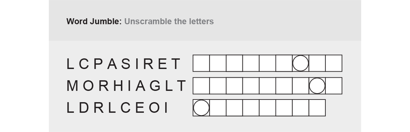
Think about that newspaper mainstay, the word jumble. The puzzle tells you which letters you need and how long the word is supposed to be. If you were lazy, you could have a computer write down the letters in every possible order, then skim through the list. Eventually you would find a word that made sense, and you would have your solution.

The list of possibilities can be quite long, though. Luckily in physics, we start with hints. We begin with an alphabet of logarithms that describe the properties our particles can have, such as their energy and speed. Then we start writing words in this alphabet, representing integrals that might show up in the final answer. Certain words do not make physical sense: they describe particles that do not actually exist or diagrams that would be impossible to draw. Others are needed to explain things we already know: what happens when a particle gets very slow or very fast. In the end, we can pare things down from what might have been millions of words to thousands, then tens, and finally just one unique answer. Starting with a guess, we end up with the only possible word that can make sense as our scattering amplitude.

Lance J. Dixon, James M. Drummond and Johannes Henn used this technique to find the right “word” for a three-loop calculation in 2011. I joined the team in 2013, when I snuck away from graduate school on Long Island to spend the winter working for Dixon at SLAC National Accelerator Laboratory at Stanford University. Along with then grad student Jeffrey Pennington, we got the result into a form we could compare with the old two-loop calculation from Del Duca, Duhr and Smirnov. Now instead of 17 pages, we had a formula that was 800 pages long—and all without drawing a single Feynman diagram.

Since then, we have pushed to even more loops, and our collaboration has grown, with Duhr, Andrew McLeod, Simon Caron-Huot, Georgios Papathanasiou and Falko Dulat joining the team. We are at seven loops, and I do not know how many pages the new formulas will take to write out. Goncharov’s trick is not enough to simplify the result when the calculation is this complicated. Here we are just happy it makes the calculation possible! We store our results in computer files now, big enough that you would think they were video files, not text.

The elliptic frontier

Recall that the more loops you include in your scattering amplitude calculation, the more precise your prediction will be. Seven loops would be more precise than the two or so loops the LHC can measure, more precise than the four-loop state of the art in quantum electromagnetism. I say “would be” here, though, because there is a catch: our seven-loop calculations use a “toy model”—a simpler theory of particle interactions than any that can describe the real world. Upgrading our calculations so they describe reality will be difficult, and there are numerous challenges. For one, we will need to understand something called elliptic integrals.

The toy model we use is very well-behaved. One of its nicer traits is that for the kind of calculations we do, Goncharov’s method always works: we can always break the integral up into an alphabet of logarithms, of integrals over circles. In the real world, this tactic runs into problems at two loops: two integrals can get tangled together so they cannot be separated.

Think about two hooked rings that cannot be pulled apart. If you move one ring around the other, you will draw a doughnut shape, or a torus. A torus has two “periods,” two different ways you can draw a line around it, corresponding to the two different rings. Integrate around a circle by itself, and you get a logarithm. Try to draw a ring around a torus, and you will not always get a circle: instead you might get an ellipse. We call such integrals around a torus elliptic integrals—integrals over an elliptic curve.

Understanding elliptic curves involves some famously complex mathematical problems. Some of these problems are so difficult to solve that organizations like the National Security Agency use them to encode classified information, on the assumption that no one can solve them fast enough to crack the code. The problems we are interested in are not quite so intractable, but they are still tricky. With the LHC’s precision increasing, though, elliptic integrals are becoming more and more essential, spurring on groups around the world to tackle the new mathematics. The machine shut down in late 2018 for upgrades, but scientists still have hordes of data to sort through; it will start up again in 2021 and will go on to produce 10 times more collisions than before.

At times the speed at which the field is moving leaves me breathless. Last winter I holed up at Princeton University with a group of collaborators: McLeod, Spradlin, Jacob Bourjaily and Matthias Wilhelm. Within two weeks we went from a sketched-out outline to a full paper, calculating a scattering amplitude involving elliptic integrals. It was the fastest I have ever written a paper, and the entire time we worried that we were going to be scooped, that another group would do the calculation first.

We did not end up getting scooped. But not long after, we received a bit of an early Christmas present: two papers by Duhr, Dulat, Johannes Broedel and Lorenzo Tancredi that explained a better way to handle these integrals, building on work by mathematicians Francis Brown and Andrey Levin. Those papers, along with a later one with Brenda Penante, gave us the missing piece we needed: a new alphabet of “elliptic letters.”

With an alphabet like that, we can apply Goncharov’s trick to more complicated integrals and start to understand two-loop amplitudes, not just in a toy model but in the real world as well.

If we can do two-loop calculations in the real world, if we can figure out what the Standard Model predicts to a new level of precision, we will get to see if the LHC’s data match those predictions. If it does not, we will have a hint that something genuinely new is going on, something our theories cannot explain. It could be the one piece of data we need to move particle physics to the next frontier, to unlock those lasting mysteries we cannot seem to crack.

*Editor's Note (2/27/19): This graph was corrected after posting. The original in the print edition inaccurately represented the curve for cosine (x).